The lognormal distribution is a commonly used distribution for modelling asymmetric data. It’s just the log of a Normal distribution right? Well no, it’s actually the other way around. You take the log of a lognormal distribution to arrive at a normal distribution. Is it just me, but I always have a bit of a mental block about this, it always feels a bit back to front.
In this post I will explore the relationship between a lognormal distribution and a normal distribution.
Generating Distribution Data
JMP has a collection of functions for generating random data sampled from a specific distribution:
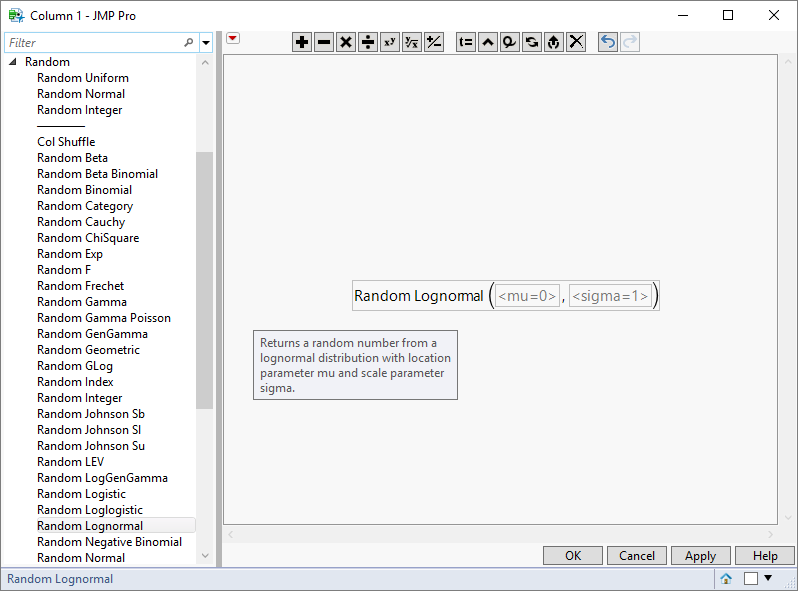
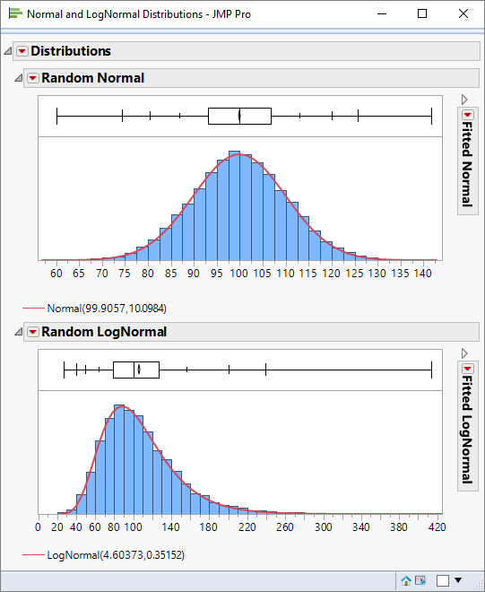
So it’s easy for me to generate data for both a normal and lognormal distribution, and to compare them:
Distribution Parameters
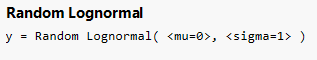
Now that I can look at the lognormal distribution let me take a closer look at its parameters. To generate random data from a lognormal distribution I use the following function:
Here is the distribution using mu=4.6 and sigma=0.35:
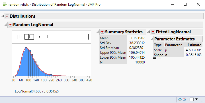
What I find confusing is that sigma is not the standard deviation of the data and mu is not the mean. Presumably then, they relate to the parameters of the associated normal distribution. Let’s see. I can create a new variable Z which is the log transform of the data:
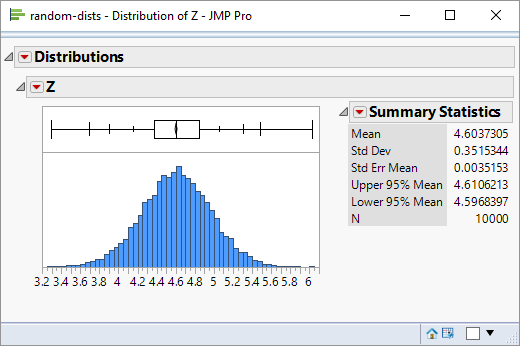
Hey presto – the mean and standard deviation match the parameters I used for the Random Lognormal function.
But What If . . .
. . . I want to generate a lognormal distribution and I want to specify the values for the mean and standard deviation? Let me take a specific example:
I want to generate a lognormal distribution with the same mean and standard deviation as the above data.
The calculation is more complex than you might expect. If 
}^2 } } \Bigg)")
 }^2 \bigg)")
Applying these equations to the above data yields values of -0.005 and 0.1 respectively.
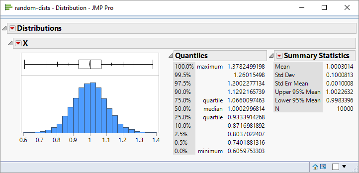
Finally, I can verify these numbers by using them with the Random Lognormal function to generate some sample data. If I have the correct parameters then the data will have a mean of 1.0 and a standard deviation of 0.1:

Very timely, thanks.
Good the hear!
Thanks for that clarification. I tried creating some random variates for a lognorm where I wanted the resulting distribution to have a mean of $1.26B and stdev $500M. I tried your method to create 100,000 rv’s, and my resulting distribution has a mean of $1.18B and a stdev of $173M. I have triple checked my formulae for the parameters. Should I expect this kind of difference? I thought maybe JMP changed the way they parameterized the lognormal. Any ideas? Thanks
There is an error with my equation.
Where it says sigma = log(…) it should be sigma-squared i.e. it is the formula for the variance rather than the standard deviation.
With this correction I have applied it to your scenario:
parameters for random lognormal function:
mu = 20.8812
sigma = 0.38241
resultant data has
mean = 1.26e9
standard deviation = 498991234