Reverse Process Capability

Process capability is a well-established technique for evaluating the degree to which a process is capable of delivering a product within specification. But what if the specifications are unknown or at best tentative?

The calculations of process capability analysis can be reversed so that for a given set of target capability values the associated specification limits can be generated. The calculation is straight-forward for a normal distribution but needs a bit more thought when it comes to asymmetric distributions.

Reverse Calculation for a Normal Distribution

Traditionally process capability is defined with respect to a normal distribution. The capability index is the ratio of the specification width to process width:

$C_p =$ $\frac{USL - LSL}{6 \sigma}$

Where σ is the standard deviation of the process variation and two-sided spec limits (USL,LSL) are assumed. The width of the specification window can be identified simply by rearranging the above formula:

$USL - LSL = 6 \sigma C_p$ $\linebreak$

In the case where we haven’t established our spec limits then we can substitute a target value for Cp to generate the width of the specification window (USL-LSL).

If our spec limits are symmetric with respect to our target, and the process is on-target, then the symmetry can be used to determine the levels of the lower and upper specs:

$USL = TGT + 3 \sigma C_p$ ,

$LSL = TGT - 3 \sigma C_p$ $\linebreak$

Where TGT represents our process target. I’ve used the ‘target’ superscript to make it more explicit that I am using a Cp value that represents the target value, and not the value derived from the data.

I can illustrate this with a specific example. Suppose that we have a process with a mean value of 100 and a standard deviation of 10 and that we want to identify spec limits that would result in a Cp of 2.0.

I can simply plug the numbers into the above formulae:

$USL = 100 + (3 \times 10 \times 2.0) = 160$

$\linebreak$
$LSL = 100 - (3 \times 10 \times 2.0) = 40$

The reverse calculation requires simple algebraic operations applied to the standard definitions of process capability indices. No knowledge of statistical theory is required.

Verifying the Calculations

The above calculations can be verified by taking a (large) random sample from a normal distribution and performing a process capability study using the proposed specification limits:

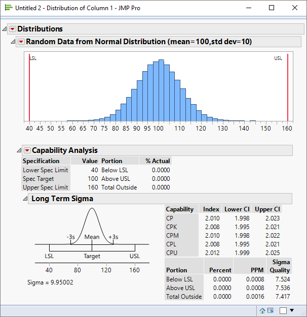
The simulation confirms that my proposed specification limits yield values a value of 2.0 for Cp.

Process Capability for Non-Normal Distributions

The reverse calculation for non-normal (asymmetric) distributions is more complex and first it is necessary to understand how the definition of capability indices is generalised for distributions such as lognormal and Weibull.

Whilst capability studies can be summarised by simple indices, they encapsulate the notion of defective parts per million. To illustrate this let’s take a simple case where we have a process on target and a process capability of 1. In this instance, by definition, the specification width is identical to the process width of 6σ.

The conversion of capability indices to dppm is dependent on the underlying distribution

We know that for a normal distribution 99.73% of the data is contained with this range. That’s another way of saying that 0.27% of data is outside of spec, equivalent to 2700 defective parts per million (dppm). The conversion of capability indices to dppm is therefore dependent on using the underlying distribution to generate probability outcomes.

Without loss of generality let’s assume that we have asymmetric process data that can be characterised using a Weibull distribution. If 6σ is the width of a normal distribution then what is the width of a Weibull distribution?

The appropriate way to define the width of the Weibull distribution is so that it has equivalent probability outcomes to the normal distribution: the width can be defined so that it contains 99.73% of the data. Furthermore this interval can be located in such a way that 0.135% of the data falls either side of this interval.

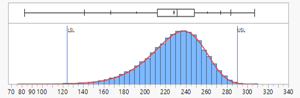
To illustrate this principle I have generated some random data sampled from a lognormal distribution and through a process of trial and error identified specification limits that satisfy the above criteria:

Reverse Calculation for the Weibull Distribution

Having established the principle for generalising capability indices I now want to explore the calculations that are required to generate proposed spec limits.

The 6σ width that we associate with a normal distribution can be generalised to an interval that contains 99.73% of the data. More specifically:

$width = P_u - P_l$

$\linebreak$

Where Pu is the upper percentile (100%-0.135%) and Pl is the lower percentile (0.135%).

This can be used to generalise the definition of process capability:

$C_p =$ $\frac{USL - LSL}{P_u - P_l}$

Furthermore the one-sided capability indices can be generalised by replacing the average value (Ybar) with the median (P50):

$C_{pu} =$ $\frac{USL - P_{50}}{P_u - P_{50}}$

and

$C_{pl} =$ $\frac{P_{50} - LSL}{P_{50} - P_l}$

Let me take the case where the process is on-target. In that case Cpl = Cpu = Cp.

Therefore

$C_{pl} =$ $\frac{P_{50} - LSL}{P_{50} - P_l}$ $= C_P$

I can rearrange this to get an expression for LSL:

$LSL = P_{50} - (P_{50} - P_l) C_p$

Taking the same approach for Cpu reveals:

$USL = P_{50} + (P_u - P_{50}) C_p$

Using Simulation to Verify the Result

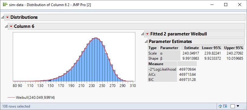
As usual I want to verify my calculations, which I can do using simulated data. The first step is for me to generate a sample of data selected randomly from a Weibull distribution:

Let me assume that my target value for Cp is 1.50. I can use this value in my expressions for the specification limits:

$LSL = P_{50} - (P_{50} - P_l) C_p^{target}$

$USL = P_{50} + (P_u - P_{50}) C_p^{target}$

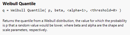
But I also need to calculate the percentiles P50, Pu and PL. I can do this using the Weibull Quantile function:

Using the alpha and beta parameter estimates from the fitted distribution I calculate the following values:

$P_{50} = 241.1$ $P_L = 123.9$ $P_U = 290.0$

Now I have all the information that I need to calculate the spec limit values required to generate my desired Cp goal. In fact let me do it as a short JSL script:

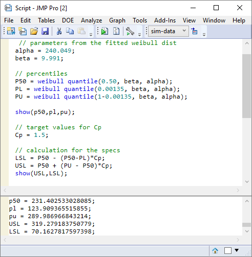
I estimate the specs to be 70 and 319.

Am I right? I can use JMP to perform the process capability analysis using these numbers:

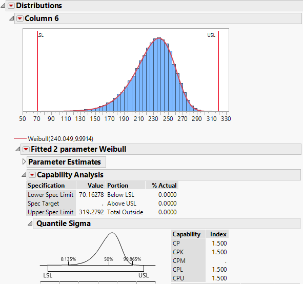
Spot on!

JMP Ahead