In my last post I introduced the idea of using the JSL script editor as a simple command line calculator; and prior to that I discussed how process capability indices (Cp,Cpk) are a convenient shorthand notation but suffer from lack of transparency. Today I will bring these two themes together by showing how I can use the JSL script editor to calculate defective parts per million (dppm) for a given set of capability indices Cp and Cpk.
Introduction
Process capability indices are a convenient way of summarising process performance. They contain information about how far a process has shifted from the mean as well as the expected number of defective parts per million. In an earlier post I showed the relationship between the capability indices and the process shift. In this post I will use the indices to calculate the expected number of defective parts per million. The calculation will involve probabilities that are calculated by reference to a Normal distribution. I will use the JSL script editor to perform these calculations.
Let’s be clear. JMP reports dppm figures when it calculates the capability indices, but nonetheless I think it’s important to understand how the information is generated rather than just blindly follow software output. As a case-study, it is also a good illustration of using the script editor to utilise the probability distribution functions available in JMP.
Framing the Problem
First I want to start with a simplified scenario where the process is on target and I can work solely with the Cp index. If the process has upper and lower specs of U and L respectively and the process standard deviation is σ then


This is the ratio of the specification window to the process width. Using 6σ as a measure of process width is just a convention: when I was first introduced to quality methods it was quite common to define the process width of 5.15σ.
Let me start with the case of Cp = 1 i.e. the spec window and the process width are identical. Now the calculation of dppm is the same as calculating the probability of an observation being outside the 6σ width.
Probability Functions
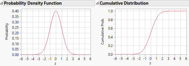
With any probability distribution (such as a Normal distribution) there are two variations in how the distribution is enumerated: a probability density function (pdf) and a cumulative probability function (cdf). In JMP the function that generates the pdf for a Normal distribution is Normal Density whereas the cdf is called Normal Distribution.
CDF Calculations
The cdf for the Normal distribution takes 3 arguments:
Normal Distribution(z, mu, sigma )
It’s good to start with a trivial test case where the answer is obvious! If I take a standard normal i.e. with mean of zero and standard deviation of 1 then I know by symmetry that 50% of the data will be less than or equal to zero:
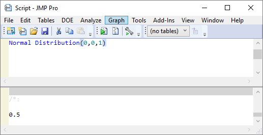
The result is a probability. Of course I could have multiplied by 100 if I wanted to explicitly express the result as a percentage or 10^6 is I wanted parts per million.
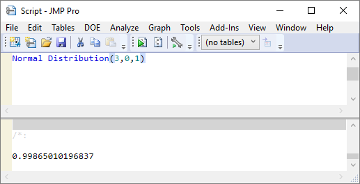
If I wanted to probability is being less than 3 standard deviations from the mean I could write:
To calculate the probability of being within the range +/- 3σ I can write: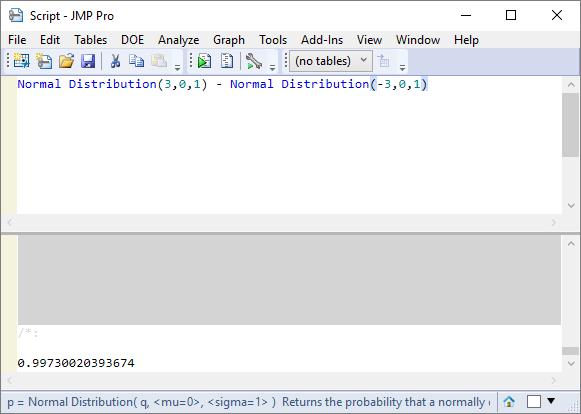
Calculating Parts per Million
With probability calculations it is often easier to calculate the logical opposite of our goal and then take one minus this value to produce the final result; this is the case with dppm calculations. In the calculation below p is the probability of being within the +/- 3σ range: so (1-p) gives me the probability of being outside the range. The 10^6 scale factor gives me the result in terms of parts per million:
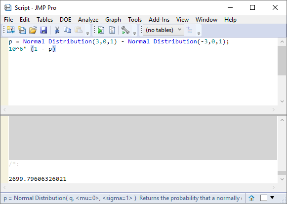
This is the well-known result that 0.27% of data is outside the 6σ width of a Normal distribution.
Recall I said that an alternative definition of the process width is 5.15σ. The motivation for this definition is that the proportion outside this process width is very close to 1% (dppm looks worse but calculations are easier!).
The Calculation for Cp = 2
Having illustrated the probability calculation for the case that the spec window is the same size as the process width, let me now take the case of Cp=2 i.e. the spec window has a width twice the process width. The width of the process is now 12σ and all I need to do is change the calculation to use a range +/-6σ:
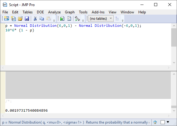
For this we need to be thinking in terms of parts per billion!
Taking Account of Process Shift
So far my calculations have assumed that I have a process on target, which allows Cp to be a sufficient descriptor of process performance. Now I want to consider both Cp and Cpk. Implicit in these two statistics is a process shift:
shift = 3σ(Cp-Cpk)
(see my previous post for the derivation of this result).
For purposes of illustration I will use the classic criteria associated with six sigma methodology: Cp=2 and Cpk=1.5. This corresponds to a process shift of 1.5.
Without loss of generality I can assume that the shift is positive in relation to the process target (which I’ll assume to be midpoint between the spec limits) as illustrated below:
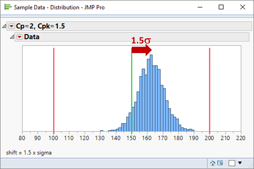
When on target the process mean is 6σ from each spec limit. With the process shift the mean is 4.5σ from the upper limit and 7.5σ from the lower limit. The number of defective parts per million will correspond to the proportion which is outside the range -7.5σ to +4.5σ:
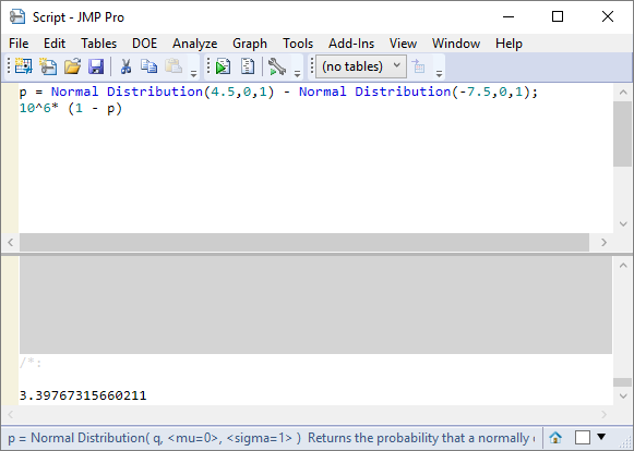
This is the benchmark result of 3.4 parts per million defective for a “six sigma “ process.