A neuron is a single node within a neural network. By analogy with neurons within the brain we can think of a neuron “firing” in response to an input trigger, and we can think of machine learning as the process of training the neuron to recognise that input trigger.
With respect to statistical modelling the activation of the neuron can be represented as a logistic model. I want to illustrate how the behaviour of a single node within a neural network is the same as a logistic model and show how networking extends the utility of the model beyond the capabilities of a single logistic representation.
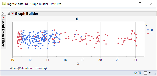
To achieve this goal I think it’s easier if I just construct some artificial data:

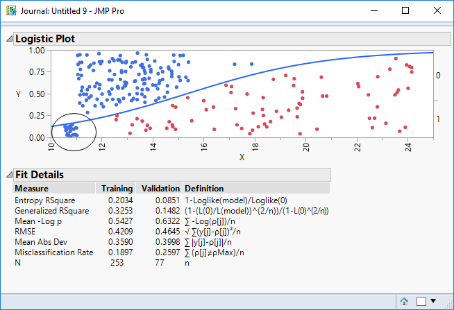
The data has been coloured by the (binary) response classification. Low values of X correspond to blue; high values correspond to red. A logistic model will transform the input X values into probability outcomes which will represent the probability associated with my target (red values);
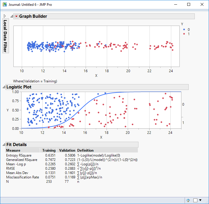
JMP output for a corresponding model representation using a neural network with a single node is shown below:
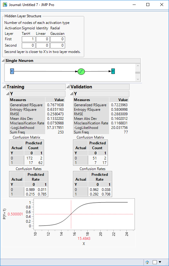
If we think of the purpose of the model as detecting “red” then both models “trigger” when X exceeds a value of about 15.5, and based on the data used to “train” the models both the logistic regression and neural network have training misclassification rates of 7.5% and validation misclassification rates of 11.7%.
Adding Complexity
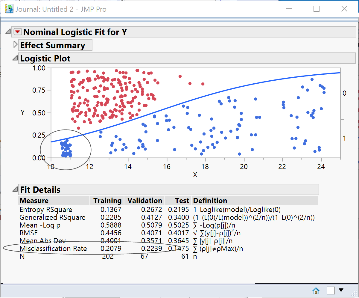
How will the two methods handle increased complexity? I’ve amended the data so that there are now some red data points for low values of X:
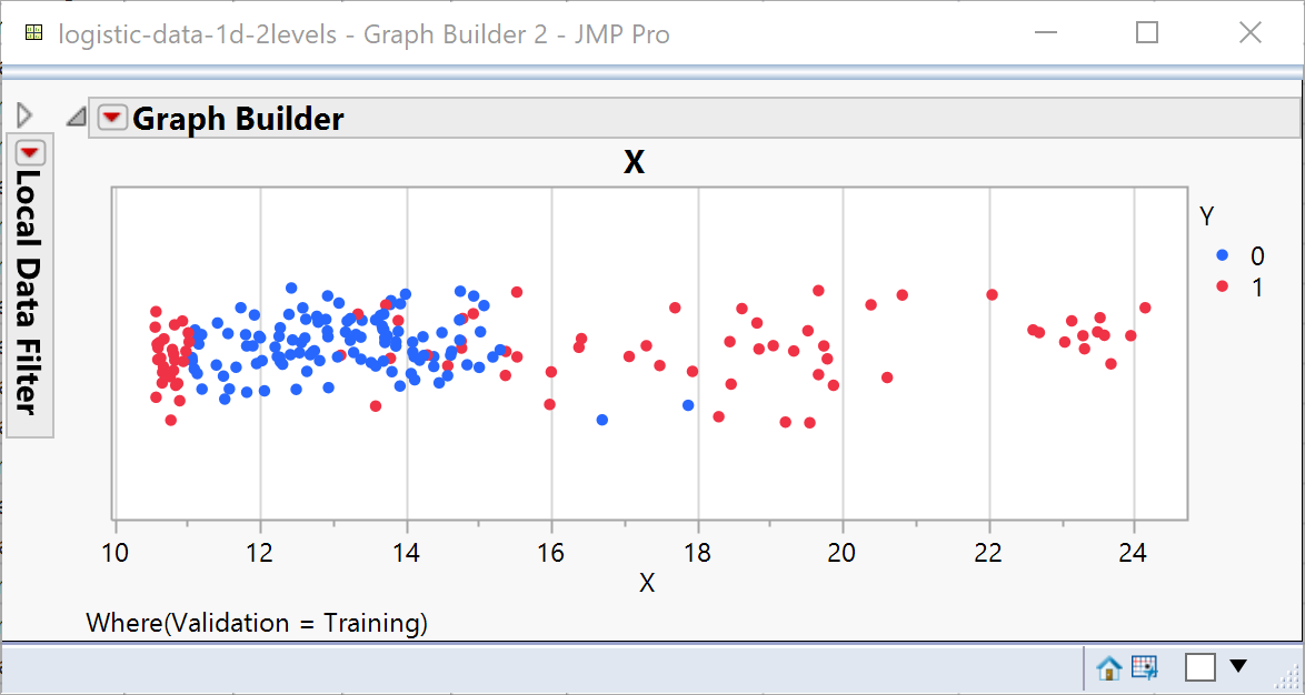
A single logistic function needs the data to transition smoothly in a single direction; all that happens is that the red data points at the low values of X become misclassified:
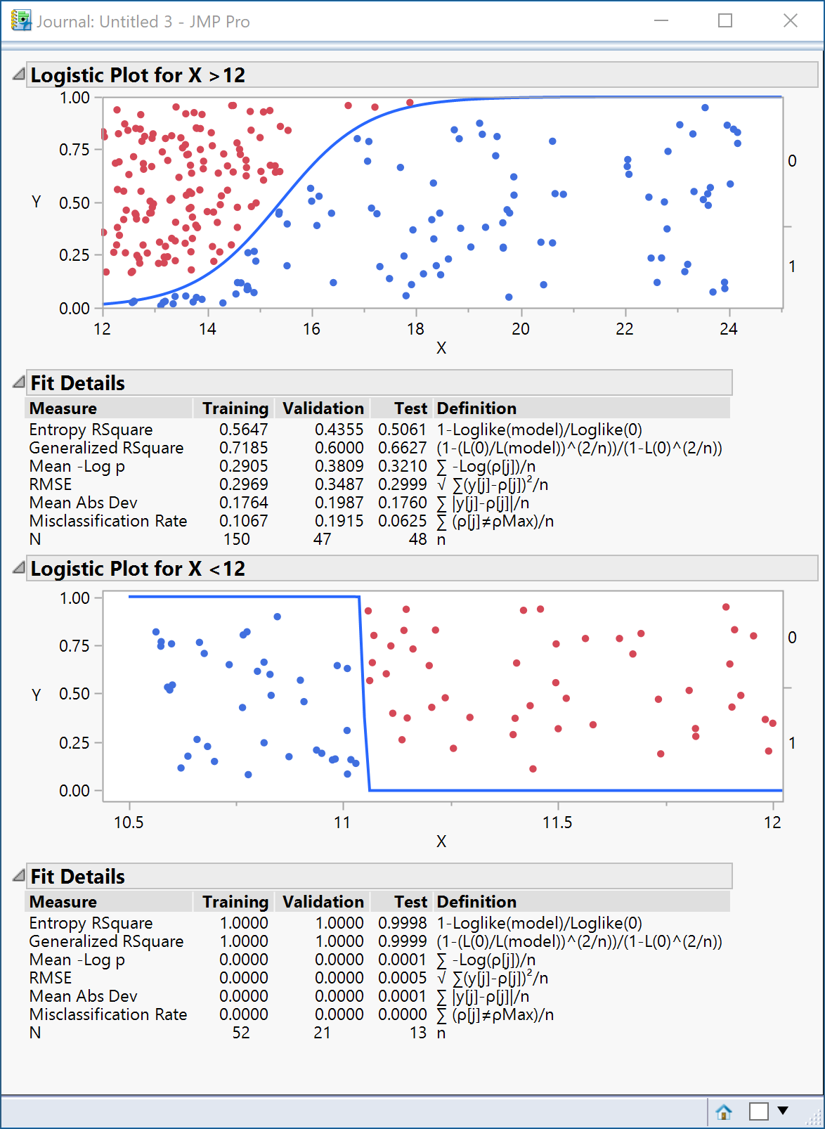
What I need to do is to build two separate models, one to model the red values at low X values and the other to model the red values for high X values. In fact I only need to build the model once and then use a global data filter to adjust the data that is being included:
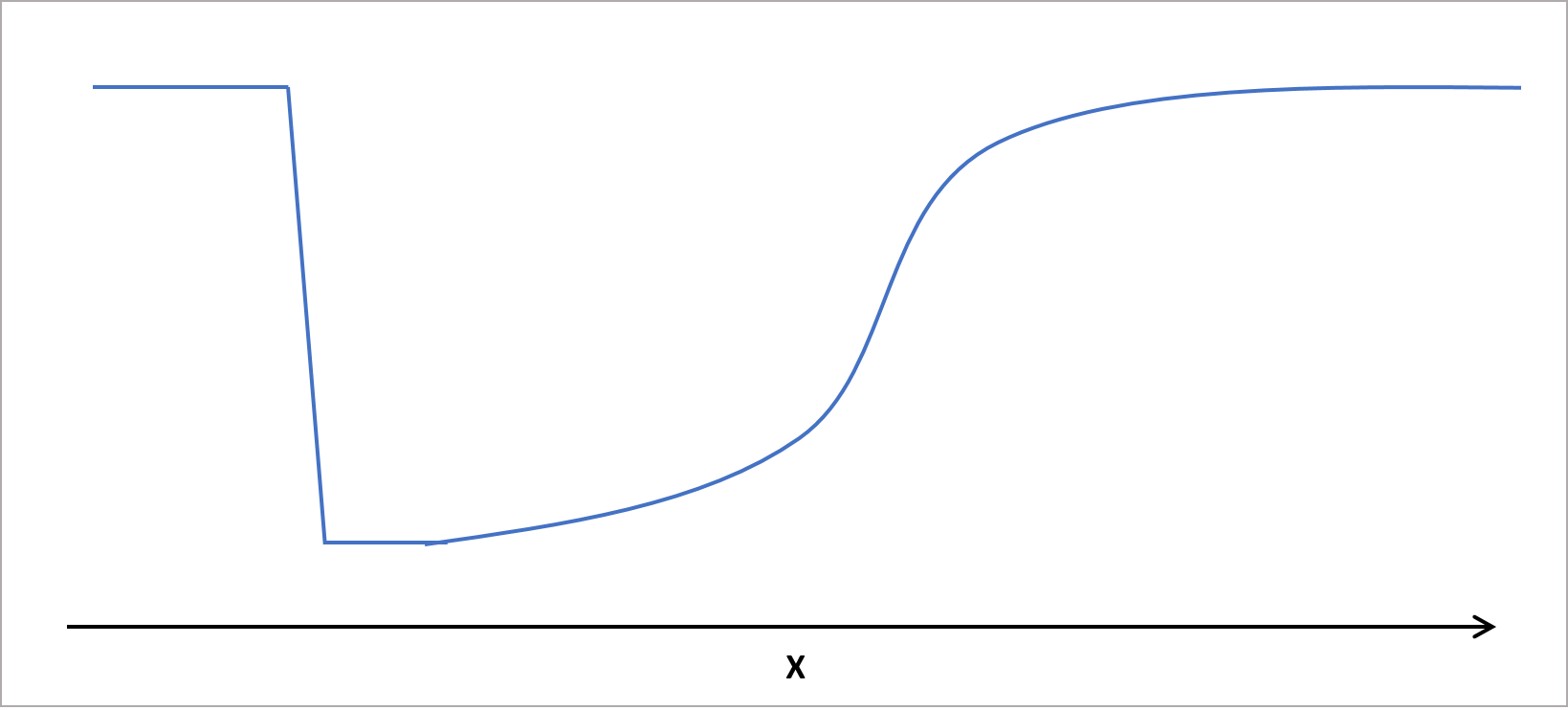
Now imagine these two models working together over the entire range of X. The prediction profile would look something like this:
For a neural network, this combination of models is achieved by having a network consisting of two neurons:
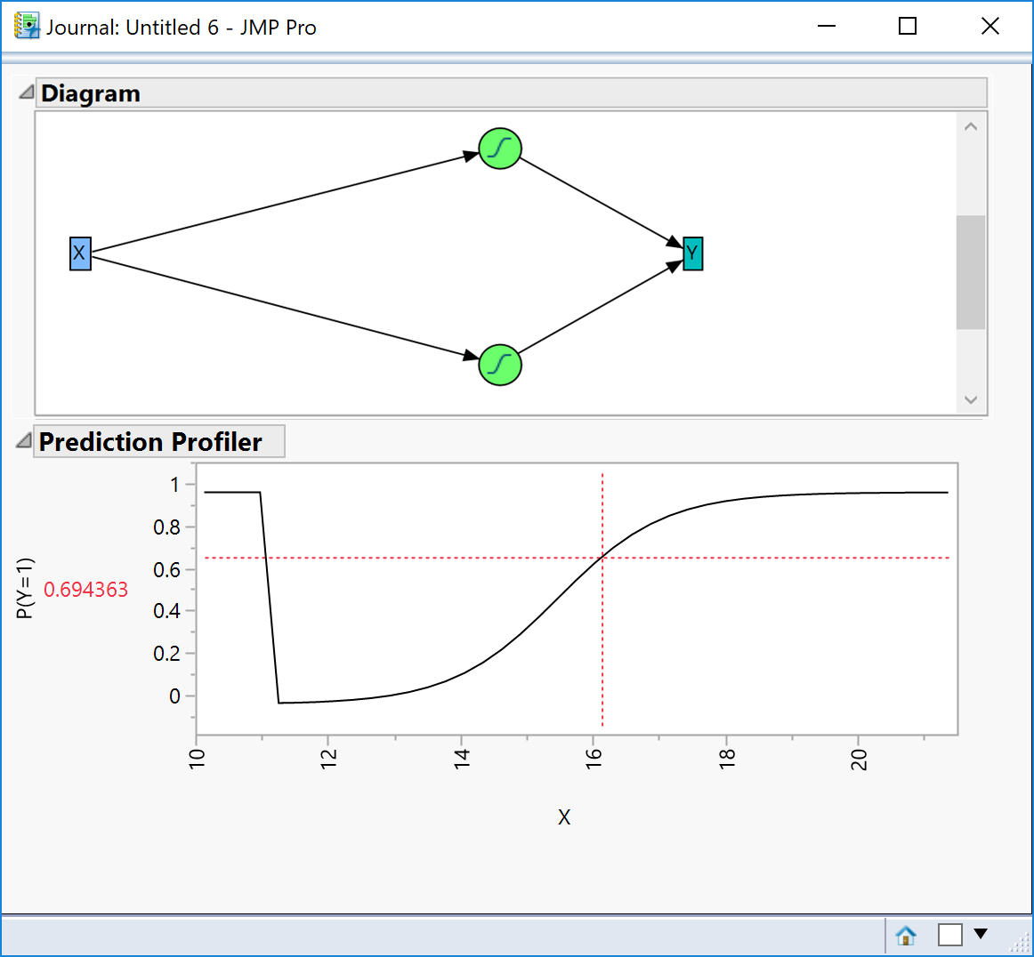
In isolation each neuron is performing a simple regression. The power of neural networks is this ability to network neurons together so that in combination they can produce a single model descriptive of the entire data, rather than having to isolate special cases and model the data separately.
Notice in particular that when I created the two logistics models, I had to look at the data and make a decision to “cut” the data at X=12. For the neural network, this point, at which the two logistic models “join”, emerges automatically from the network as observed in the prediction profiler.