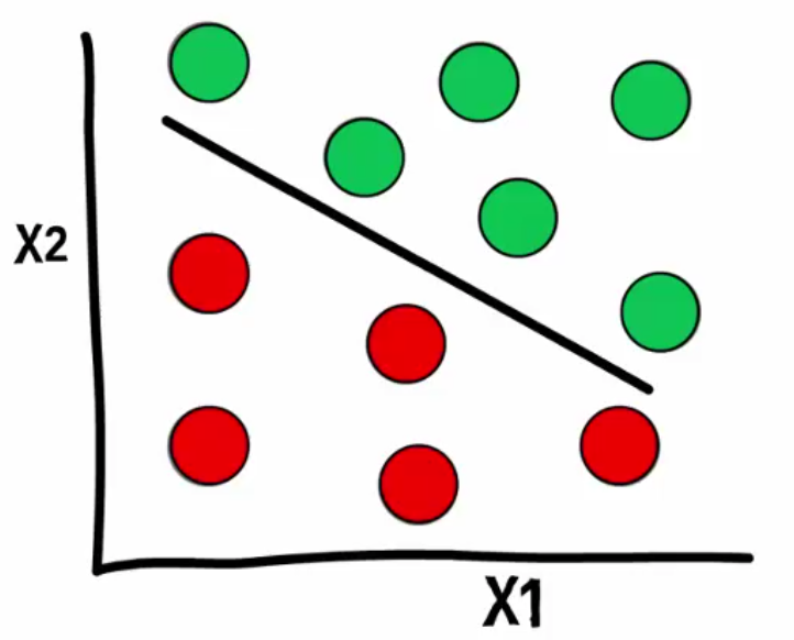
 In my last post I outlined some “homework” that I had set myself – to write a script that would create linearly separable data. I want the ability to create it in an interactive environment. But before I create the interactivity I want to get the foundations correct. So in this post I will build the code but with the interactive elements.
In the last post I identified these four key elements to the script:
- Data
- Graph
- Line
- Response
Let’s take a look at each of these in turn.
1. Data
The start point is to create a data table containing columns for two input variables (X1 and X2) and a binary response (Y).
|
1 2 3 4 5 6 7 8 9 10 11 12 13 14 15 16 17 18 19 20 21 22 23 24 25 |
Names Default To Here(1); // create X1 and X2 data and set colour // properties for binary response nDataPoints = 100; dt = New Table("Linearly Separable Data", Add Rows(nDataPoints), New Column("X1", Numeric, Continuous, Format( "Fixed Dec", 10, 2 ), Set Formula( Random Uniform() ) ), New Column("X2", Numeric, Continuous, Format( "Fixed Dec", 10, 2 ), Set Formula( Random Uniform() ) ), New column("Y", Numeric, Nominal, Set Property( "Value Colors", {-1 = 3, 1 = 4) ) ); |
Lines 5 & 7
The number of data points in the table have been set as a variable so that this can be easily changed (and ultimately specified by the user.
Lines 6 to 25
This is the New Table function. If it looks like a lot of code that’s just because I have put each New Column field on a separate line. It could have been written like this:
|
1 2 3 4 5 6 |
dt = New Table("Linearly Separable Data", Add Rows(nDataPoints), New Column("X1", Numeric, Continuous, Format( "Fixed Dec", 10, 2 ),Set Formula( Random Uniform() ) ), New Column("X2", Numeric, Continuous, Format( "Fixed Dec", 10, 2 ),Set Formula( Random Uniform() ) ), New column("Y",Numeric, Nominal, Set Property( "Value Colors", {-1 = 3, 1 = 4} )) ); |
– more compact but ultimately less readable.
Lines 12 & 18
The function Random Uniform generates random numbers uniformly from the range 0 to 1.
Lines 11 & 17
The numbers have been formatted so that they display with two decimal places. This is purely cosmetic.
Lines 20 to 24
This is the definition of the response column. The response is binary. Setting the modelling type to Nominal will assist when I want to colour the data points based on the binary value (it will prevent JMP trying to use a continuous scale for the colour).
Line 23
The Value Colors property of the column can be used to pre-assign colours to the binary levels (-1 and +1) of the response. To figure out the syntax for this property you can refer to the documentation or get JMP to do it for you:
2. Graph
The above code can be used to create a data table containing 100 rows of X1 and X2 data. Using Graph Builder a scatterplot of X2 versus X1 can be produced. Y can be applied to the Color role (even though it doesn’t yet have any data). The range of the axes can be modified to be from 0 to 1 and the marker sizes can be made as large as possible. With all of these edits JMP will create the following code (with a couple of exceptions listed below):
|
26 27 28 29 30 31 32 33 34 35 36 37 38 |
// create graph of X1 versus X2 with Y assigned as colour gb = dt << Graph Builder( Size( 500, 500 ), Show Control Panel( 0 ), Variables( X( :X1 ), Y( :X2 ), Color( :Y ) ), Elements( Points( X, Y, Legend( 17 ) ) ), SendToReport( Dispatch( {}, "X1", ScaleBox, {Min(0),Max(1),Inc(1)} ), Dispatch( {}, "X2", ScaleBox, {Min(0),Max(1),Inc(1)} ), Dispatch( {}, "graph title", TextEditBox, {Set Text( "" )} ), Dispatch( {}, "Graph Builder", FrameBox, {Marker Size( 6 )} ) ) ); |
– line numbers are based on the full script, so this block of code follows on from the data creation.
Line 26
I have added an explicit reference to the table (dt) and added a reference to the Graph Builder object, gb.
3. Line
Here is the code followed by an explanation:
|
40 41 42 43 44 45 46 47 48 49 |
// draw line: y=mx+c m = -0.4; c = 0.7; p1 = {0,c}; p2 = {1,m+c}; rep = gb << Report; fb = rep[FrameBox(1)]; fb << Add Graphics Script( Line(p1,p2) ); |
Lines 41 to 44
The equation of a line can be written as:

Drawing the line only requires the line to be evaluated at two points (p1 and p2) corresponding to X1=0 and X1 = 1 respectively.
p1 = {0,c} and p2 = {1, m+c}
Line 45
A reference to the Graph Builder window is obtained by sending the Report messsage to the Graph Builder object.
Line 46
This line obtains a reference to the FrameBox, which is the graphical region of the graph (where the markers are plotted).
Lines 47 to 49
The contents of the FrameBox can be customised by adding graphics scripts. The code uses the Line function to plot a line between the points p1 and p2.
4. Response
The line defines a boundary. Data points above the boundary need to be assigned a Y value of +1. Those points satisfy the criteria:

The data points below the line are set to -1.
Ultimately the definition of the line will be interactive (next post!) and so it is helpful if the response if defined as a formula, and the formula is based on externally defined variables. So I am going to use table variables to store the values of m and c:
|
51 52 53 54 55 56 57 58 59 60 61 |
// binary response // 1 if above line, -1 if below dt << Set Table Variable("m",m); dt << Set Table Variable("c",c); Column(dt,"Y") << Set Formula( If ( :X2 > m*:X1+c, 1 , -1 ) ); |
The Y column has already been assigned as a Color role on the graph so this formula also results in the markers being colour-coded:
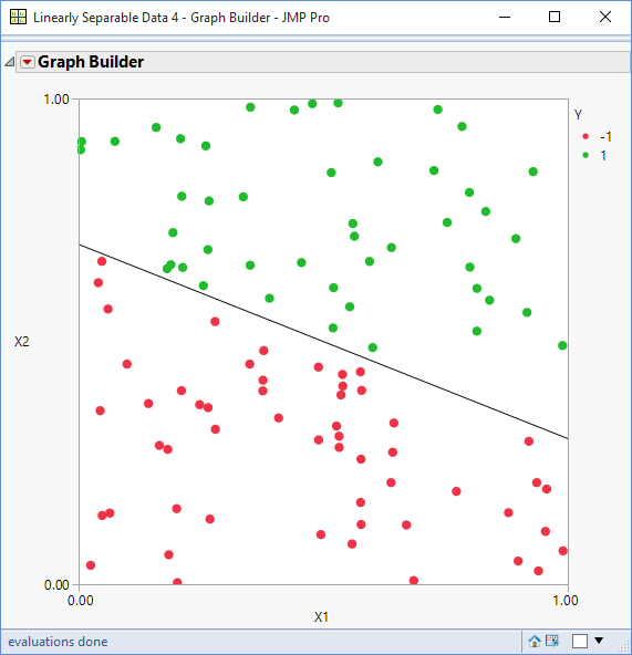
I now have a script which generates a Y column containing binary values that are separated by a straight line of abitrary orientation. In my next blog I will add “grab-handles” to the line so that the orientation can be defined interactively by the user.
Finally, here is a full listing of the code:
|
1 2 3 4 5 6 7 8 9 10 11 12 13 14 15 16 17 18 19 20 21 22 23 24 25 26 27 28 29 30 31 32 33 34 35 36 37 38 39 40 41 42 43 44 45 46 47 48 49 50 51 52 53 54 55 56 57 58 59 60 61 |
Names Default To Here(1); // create X1 and X2 data and set colour properties for binary response nDataPoints = 100; dt = New Table("Linearly Separable Data", Add Rows(nDataPoints), New Column("X1", Numeric, Continuous, Format( "Fixed Dec", 10, 2 ), Set Formula( Random Uniform() ) ), New Column("X2", Numeric, Continuous, Format( "Fixed Dec", 10, 2 ), Set Formula( Random Uniform() ) ), New column("Y", Numeric, Nominal, Set Property( "Value Colors", {-1 = 3, 1 = 4} ) ) ); // create graph of X1 versus X2 with Y assigned as colour gb = dt << Graph Builder( Size( 500, 500 ), Show Control Panel( 0 ), Variables( X( :X1 ), Y( :X2 ), Color( :Y ) ), Elements( Points( X, Y, Legend( 17 ) ) ), SendToReport( Dispatch( {}, "X1", ScaleBox, {Min(0),Max(1),Inc(1)} ), Dispatch( {}, "X2", ScaleBox, {Min(0),Max(1),Inc(1)} ), Dispatch( {}, "graph title", TextEditBox, {Set Text( "" )} ), Dispatch( {}, "Graph Builder", FrameBox, {Marker Size( 6 )} ) ) ); // draw line: y=mx+c m = -0.4; c = 0.7; p1 = {0,c}; p2 = {1,m+c}; rep = gb << Report; fb = rep[FrameBox(1)]; fb << Add Graphics Script( Line(p1,p2) ); // binary response // 1 if above line, -1 if below dt << Set Table Variable("m",m); dt << Set Table Variable("c",c); Column(dt,"Y") << Set Formula( If ( :X2 > m*:X1+c, 1 , -1 ) ); |
Maintain the excellent job !! Lovin’ it!