Curve Fitting

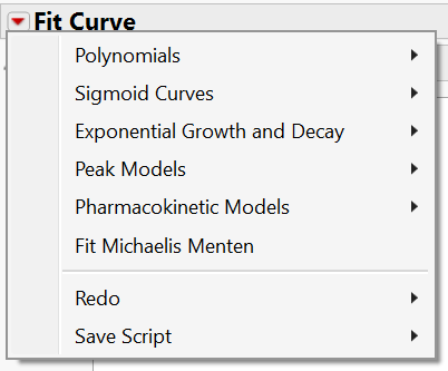
The curve fitting platform allows you to select from a library of model types.

In this post I take a closer look at the different model types that are available to support curve fitting.

Each of the model categories contain a variety of models with differing numbers of parameters:

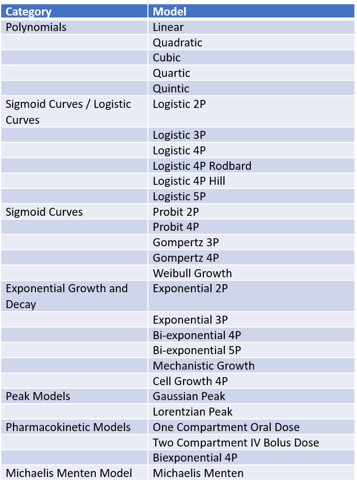
Polynomial Models

If you use linear regression (standard least squares) you will be familiar with this type of model:

$y=\ \beta_0+\ \beta_1\ x+\ \beta_2\ x^2+\ \beta_3\ x^3\ \ +$ . . .

Whilst gradient descent algorithms can be used to estimate these parameters, the primary role of curve fitting is to fit parameters that form part of a nonlinear equation – typically representing some mechanistic model relating to a scientific application. All other model types fall into this category of nonlinear models.

Sigmoid / Logistic Curves

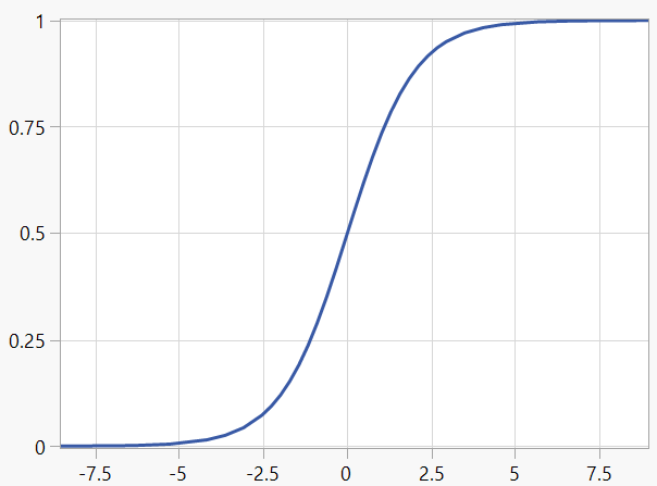
The basic sigmoid function takes the following form:

$y =$ $\frac{1}{1 + e^{-x}}$

It characterises the case where an unbounded x variable is transformed into a y variable that is contained within a range 0 to 1. It is therefore particularly useful for modelling a response that represents a proportion.

The logistic function introduces one or more parameters to generalise the behaviour of this S-curve. For example, a parameter can be introduced to control the growth rate:

$y =$ $\frac{1}{1 + e^{-a \cdot x}}$

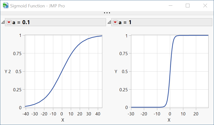
The curve has a point of inflection at x=0. The introduction of a second parameter allows the location of this inflection point to be adjusted:

$y =$ $\frac{1}{1 + e^{-a \cdot (x-b)}}$

This is the formula for the Logistic 2P model.

Whilst y is a continuous response, these types of model are often used to model a binary outcome (0 or 1). In this case the y value is interpreted as the probability of an outcome of 1 given a specified value of x.

The Logistic 3P model introduces a third parameter allowing the curve to have an upper asymptote other than 1:

$y =$ $\frac{c}{1 + e^{-a \cdot (x-b)}}$

And the Logistic 4P model provides a description of both upper and lower asymptotes with parameters c and d:

$y = d +$ $\frac{c-d}{1 + e^{-a \cdot (x-b)}}$

There is also a Logistic 5P model that allows the curve to be asymmetric about the inflection point:

$y = d +$ $\frac{c-d}{[{1 + e^{-a \cdot (x-b)}}]^f}$

Sigmoid/Probit Curves

The logistic functions described earlier typically represent the case where the response is derived from the probability of a binary outcome. Alternatively, we can model the S-curve on the basis that it represents the cumulative distribution function Φ of a Normal distribution:

$y = \Phi$ $(\frac{x-b}{a})$

where the parameter a represents the growth rate and b is the point of inflection. This is the Probit 2P model.

The Probit 4P model introduces parameters to control the lower and upper asymptotes:

$y = c+(d-c)\cdot\Phi$ $(\frac{x-b}{a})$

Sigmoid/Gompertz Curves

The 5-parameter logistic model describes an S-shaped curve that is asymmetric about the inflection point. A Gompertz curve can be considered to be a special case of this model. As described in Wikipedia the model was first proposed as a description of human mortality.

$y = a\cdot e^{-e^{-b(x-c)}}$

A four-parameter model is also available that provides parameters for both lower and upper asymptotes.

Sigmoid/Weibull Growth Curve

Another S-shaped curve is the Weibull Growth model, often used in reliability engineering:

$y = a[1-e^{-(x/c)^b} ]$

Where a is the upper asymptote, b is the growth rate, and c is the inflection point.

Exponential Growth and Decay

Exponential 2P is the basic exponential model:

$y = b\cdot e^{\lambda \cdot x}$

The parameter b is a scaling parameter and λ represents the growth rate. If λ is negative, then it represents the rate of decay.

The Exponential 3P model adds an additive term to control the asymptote of the curve:

$y = a+b\cdot e^{\lambda \cdot x}$

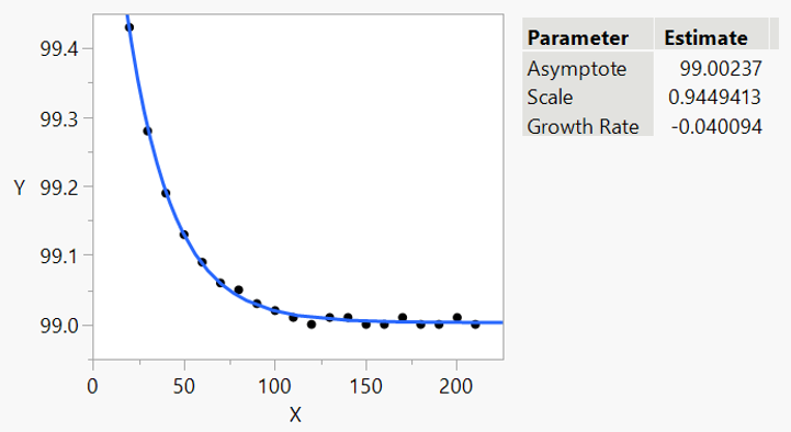
An alternative parameterisation is the mechanistic growth model:

$y = a(1-b\cdot e^{\lambda \cdot x})$

JMP also supports bi-exponential models. These models are the sum of two exponentials and appear as 4-parameter and 5-parameter models:

$y = a\cdot e^{-b \cdot x}+c\cdot e^{-d \cdot x}$

$y = a+b\cdot e^{-c \cdot x}+d\cdot e^{-e \cdot x}$

Cell Growth

Growth of cells in a bioreactor can be characterised by a number of phases:

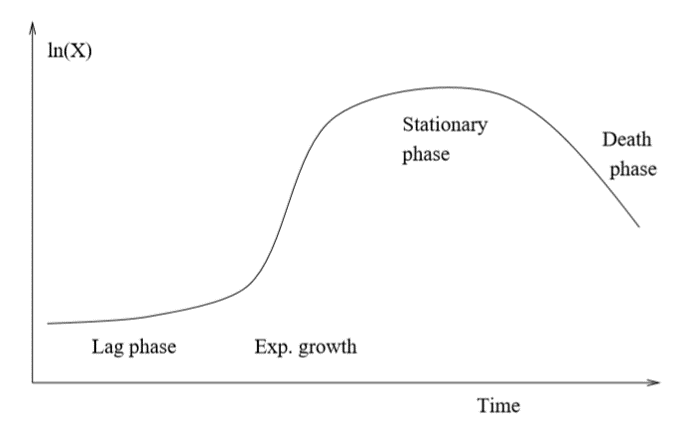
JMP’s Cell Growth 4P model takes the form:

$y = \frac{ab}{(a-b) e^{-c \cdot x}+b e^{d \cdot x}}$

where:

a = peak value if mortality rate is zero
b = response at time zero
c = cell division rate
d = cell mortality rate

Peak Models

The bell-shaped curve associated with a Normal distribution is more generically described by a Gaussian function of the form:

$y = ae^{\frac{(x-b)^2}{2c^2}}$

The Lorentzian curve is superficially similar to the Gaussian bell-shape, but has heavier tails:

$y = \frac{ab^2}{(x-c)^2+b^2}$

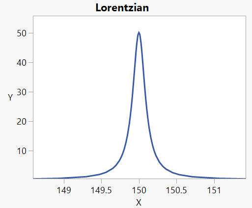
Peak curves are used, for example, to model spectroscopic peaks.
For both models the parameter a corresponds to the maximum value of the peak; b represents the growth rate, and c is the critical point: the value of x where the curve reaches its maximum value.

Pharmacokinetic Models

Pharmocokinetic models seek to describe the kinetics of a drug once it has been administered into the body. The One Compartment Oral Dose model has the following parameterisation:

$y = \frac{abc}{c-b}(e^{-b\cdot x}-e^{-c\cdot x})$

where:

a = area under the curve
b = elimination rate
c = absorption rate

JMP also supports a Two Compartment IV Bolus Dose model, but that is beyond my latex skills!

Michaelis-Menten Model

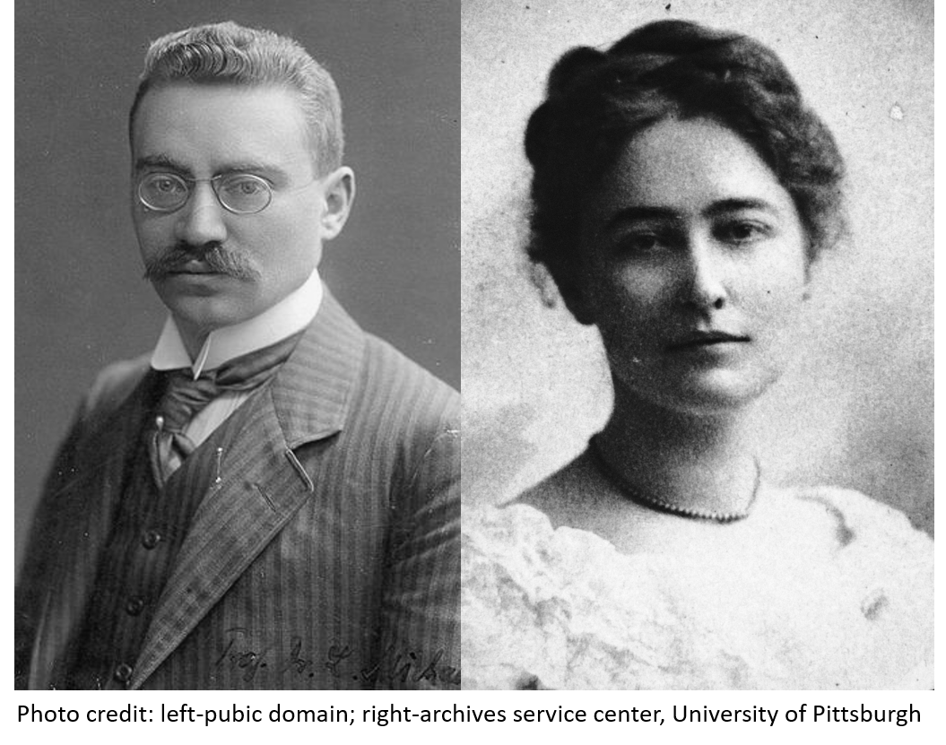
Named after the biochemists Leonor Michaelis (1875-1949) and Maud Menten (1879-1960), this model is used to describe enzyme kinetics:

$y = \frac{ax}{b+x}$

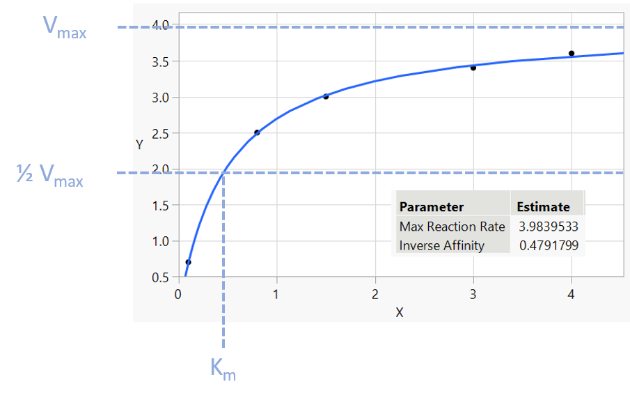
The parameter a represents the maximum reaction rate (in literature often referred to as V_max), and the b parameter (in literature often referred to as the Michaelis constant K_m) is the value of x such that the response is half V_max ; it is an inverse measure of the substrates affinity for the enzyme.

And There Is More

We are not limited to selecting from a pre-defined library of curve types. Any nonlinear function can be expressed as a column formula and fitted using the Nonlinear Platform. In fact it is one of my most frequently used platforms. But that is a topic for another day.

2 thoughts on “Curve Fitting”

Alonso Romero says:

July 19, 2022 at 11:57 am

Interesting explanation. At this moment, I’m analysing some data using some Fit Curves in JMP. I’m finding that my data fit when I’m using a Logistic 3P model. But my question is the following: What are the equations or the way that JMP determines the growth rate (a), the inflexion point (b), and the asymptote?

1. David Burnham says:
  
  February 15, 2023 at 2:54 pm
  
  JMP seeks to find parameter estimates that minimise the sum of squares of the residuals. That’s the same goal as standard least squares, but for nonlinear models this is achieved by minimising a loss function. The minimisation procedure involves taking first and second order derivatives and setting them to zero. The procedure shares similarities with the Newton-Raphson method.

JMP Ahead