In a recent post I created a table that contained two classes of data: images that represent either the handwritten digit ‘5’ or the digit ‘6’. In this post I’ll model the data using logistic regression. I will also take the opportunity to look at the role of training and test datasets, and to highlight the distinction between testing and validation.
The Logistic Function
The most common form of regression is linear least-squares regression. This model-form is used when the response variable is continuous. When it is discrete the equivalent modelling technique is logistic regression.
To understand logistic regression it is helpful to be familiar with a logistic function. The standard logistic function takes the following form:

This function plots as an S-shaped (sigmoidal) curve:
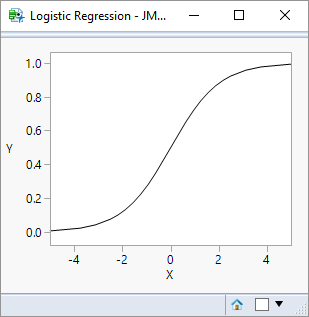
A useful characteristic of the curve is that whilst the input (X) variable may have an infinite range, the output (Y) is constrained to a range 0 to 1. This makes it particularly useful for representing probability responses.
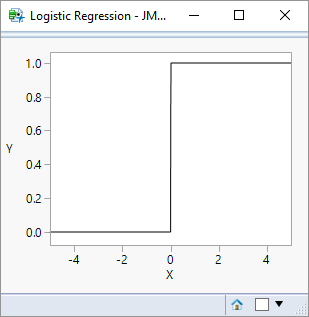
For a binary classification problem such as the fives-and-sixes classification, the curve can be used to represent the probability (p) of one of the classes: the probability of the other class is simply 1-p. The most probable class is therefore the one with a probability greater than 50%; in this way the logistic function can be used to describe either a continuous probability outcome or a discrete binary outcome. Ideally, we identify parameters (beta) and features (X) that provide a clear distinction between the classes. Below is the same function but using a parameter value (beta) of 1000:
Creating My Predictor Variables
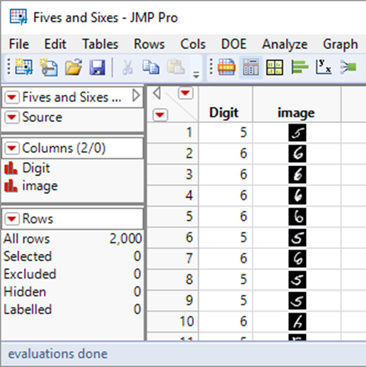
My response variable is clear: it is my digit column that contains the classification value 5 or 6 (see my last blog for further details).
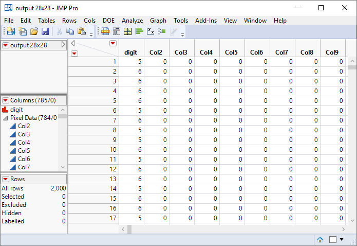
But what about my X variables that will describe the features within the images? I’m going to start with the raw pixel data. So for each row of the table, I want to create a column for each pixel in the image. I know that the images are 28×28, so that means that there will be 784 columns of pixel data.
Here is a script to do the hard work of creating these columns:
|
1 2 3 4 5 6 7 8 9 10 11 12 13 14 15 16 17 18 19 20 21 22 23 24 |
dt = Current Data Table(); imageCol = Column(dt,"image"); // get a sample image to determine size img = imageCol[1]; {x,y} = img << Get Size; size = x*y;s nr = NRows(dt); m = Matrix(nr,1+size); m[1::nr,1] = Transpose(Column(dt,"Digit")[1::nr]); For (i=1,i<=nr,i++, img = Column(dt,"image")[i]; p = img << Get Pixels; s = Shape(p,1,size); {cr,cg,cb} = Color To RGB(s); m[i,2::size+2-1] = cr; ); ndt = New Table("output " || Char(x) || "x" || Char(y), <<Set Matrix(m)); Column(ndt,1) << Set Name("digit"); Column(ndt,1) << Set Modeling Type("nominal"); cols = ndt << Get Column Names(String); RemoveFrom(cols,1); ndt << Group Columns("Pixel Data",cols); |
The new columns have been placed in a column group Pixel Data:
Building the Model
When you use the Fit Model platform with a response variable that has a nominal modelling type JMP automatically selects the logistic personality. In this instance digit is the response. For my predictor variables I can use one or more of the Pixel Data columns.
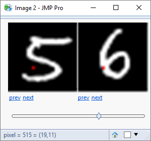
I’ll start with a single variable. I’m going to use column 216 – that corresponds to a pixel that i believe should be “on” for a five, and “off” for six. I’ve highlighted the pixel as the red point below:
![]()
There are of course counter-examples:
![]()
But on the balance of probabilities it looks like a reasonable selection. The logistic model will evaluate that balance of probabilities.
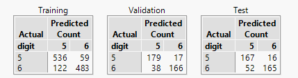
The output from a logistic model can look intimidating – so I am going to focus on just one piece of information – the confusion matrix:
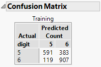
My data table contains 2000 rows – 974 (48.7%) fives and 1026 (51.3%) sixes.
So roughly speaking if I were to make a random guess of the value of a digit I would have a 50:50 chance of being correct. Using the model I would like my chance of success to be “lifted”. So what does the confusion matrix tell me? The model does a fairly good job of classifying the sixes correctly and gives me a better than evens chance of predicting a five.
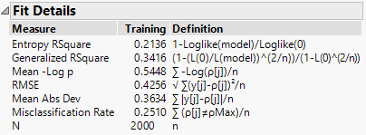
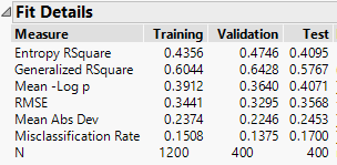
On balance 502 (119+383) of the 2000 data points were misclassified. This is a misclassification rate of 0.25: a statistic that is reported in the Fit Details outline:
Considering that I am only using one pixel, I’m very happy with that. But two questions come to mind:
- Have I made a fair evaluation of the model?
- Could I have chosen a better pixel?
I will look at these questions in turn. They will introduce the idea of partitioning data for the purposes of model tuning and predictive evaluation.
Have I Made a Fair Evaluation of the Model?
The short answer is no. This is easier to explain by analogy with a simple linear regression. If I take two data points and fit a line through them then clearly the line will go through those points. I can’t use the “goodness of fit” of those points to evaluate the predictive capability of the model. What I need to do is hold back some of the data so that it is not used in the modelling process. Once I have a model I can use it to predict the values of the data that was unseen during the modelling process. It is usual terminology to refer to the data used for modelling as the training dataset and the held-back data as the test dataset.
JMP software allows me to designate a column that contains a flag that differentiates between the different datasets. The training dataset is used for modelling, but separate output is produced for both my training and test datasets:
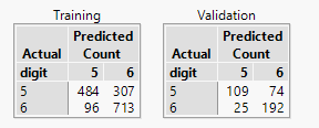
On the left are the results for the training data. This should be similar to what I had before, although I am now only using 1600 rows of the data (80%). The remaining 20% of the rows are my training dataset (ignore the fact the JMP wants to call it a validation dataset!).
Similarly the Fit Details outline now summarises the misclassification rates for each dataset:
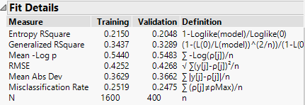
My test dataset (“validation”) is reporting a misclassification rate of 25% – consistent with the results that I get from the data used to build the model. So I’m happy that that is a fair reflection of the model performance.
As a side-note: this is not a surprise. The rationale of using a test dataset is to protect against overfitting. But this model only contains a single predictor variable. In future posts I’ll be looking at more complex models where I need to protect against overfitting.
Could I Have Chosen a Better Pixel?
The short answer is “probably”. I chose a pixel based on some common sense and a visual inspection of the data. Now I’m going to try a brute force approach – the following script will build a model based on each of the 784 pixels:
|
1 2 3 4 5 6 7 8 9 10 11 12 13 14 15 16 17 18 19 20 21 22 23 24 25 26 27 28 29 30 |
dt = Current Data Table(); lstNames = {}; lstTrainingRates = {}; lstTestRates = {}; For (i=2,i<=785,i++, cName = Column(dt,i) << Get Name; fm = Fit Model( Y( :digit ), Effects( Eval(cName) ), Validation( :Validation ), Personality( "Nominal Logistic" ), Run( Likelihood Ratio Tests( 1 ), Wald Tests( 0 ), Logistic Plot( 1 ) ), SendToReport( Dispatch( {}, "Fit Details", OutlineBox, {Close( 0 )} ) ) ); model = fm << Get Scriptable Object(); rep = model << Report; mat = rep[NumberColBox(15)] << Get As Matrix; trainingRate = mat[6]; mat = rep[NumberColBox(17)] << Get As Matrix; testRate = mat[6]; InsertInto(lstNames,cName); InsertInto(lstTrainingRates,trainingRate); InsertInto(lstTestRates,testRate); rep << Close Window; ); New Table("Results", New Column("Column Name", character, Set Values(lstNames)), New Column("Misclassification Rate (training)", numeric, Set Values(lstTrainingRates)), New Column("Misclassification Rate (test)", numeric, Set Values(lstTestRates)) ) |
The results suggest that pixel 515 is the best predictor with a misclassification rate less than 20% – not bad for a single pixel!
Here is the location of that pixel:
[side note: a closer inspection of the results suggests that there are 4 clusters of pixels that yield good predictive results, each cluster identifying different characteristics of the digits – top stroke, two components of the circular stroke, and the tail. ]
I have answered the two questions: “have I made a fair evaluation of the model?” and “could I have chosen a better pixel”. But in the process I have raised a third question:
“Have I made a fair evaluation of the different models used to select the best pixel?”.
The process I performed for selecting the “best” pixel is itself subject to the problems of overfitting. I am using a script to improve my model by selecting a predictor variable that maximises the model performance. I have used a test dataset to evaluate the model, but I am now using the same dataset as part of the model building process. In fact it is not testing the model, it is a component of the model “tuning” process.
I need three distinct sets of data:
Training – used to build the model (i.e. estimate model parameters)
Validation – used for tuning model parameters and differentiating between different model prototypes
Test – a true hold-back dataset used for evaluating model performance
In just the same way that JMP allowed me to have a column that identified training and test, I can use the column to identify all three classes of data (in fact, JMP prefers it – the labelling starts making sense!). Here is an example:
My script for looking at model performance can now focus on the validation results, and then I can make a final assessment of predictive performance using the test results.
Whilst I can code my script to ignore the test results I personally feel that it is impossible to see test results in the output and not have them influence the model building process. Therefore I typically remove them entirely by constructing separate tables: one for training and validation, the other for testing.
And Finally
Earlier I introduced the logistic function. So as well as looking at the confusion matrix and I can use the logistic function to get a sense of the model behaviour:
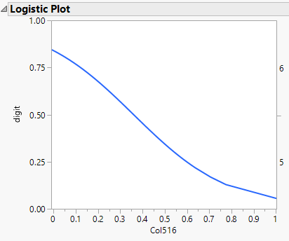
When the pixel is “off” the function has a value of about 0.8, reflecting the probability that the digit is a six. When the pixel is “on” the probability has a value of about 0.1 (equivalent to a probability of 0.9 that the digit is a five).
2 thoughts on “Logistic Regression pt.1”