An understanding of how variance propagates through a system can help us design experiments that maximise the precision of our results.
Traditionally scientists and engineers are taught how to conduct scientific experiments, then analyse the data in the context of their domain-specific knowledge (physics, chemistry, electronics, etc), and finally to apply statistical methods to calculate the precision of their results.
Statistical design of experiments reverses the sequence of data analysis, by first anticipating the precision of the results and how the precision is influenced by the experimental configuration.
By doing so, the experiment can be enhanced to yield higher precision results from the same level of experimental resource.
To illustrate this, consider a simple scenario where we have a set of scales with known measurement precision, and 3 unknown weights that we wish to measure:
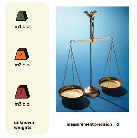
For example, the scales may have a standard deviation of 5 grams, and we measure the first weight to have a value of 80 grams:
![]()
The standard deviation represents variations that can arise in our data even though we are measuring the same “thing”.
We are often taught that to get a more precise measurement we can repeat our measurements.
The average of our measurements will have a precision improved by a factor √N where N is the number of repeats.
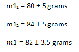
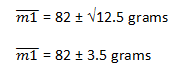
For example, imagine that we took two measurements for m1 of 80 and 84:
This improvement in precision is a result of how variance propagates through our experimental system. In general, variances are said to be additive. To illustrate this we’ll take a closer look at the calculation above for the average value of m1:
![]()
If the variance of each measurement is 25 (5×5) then the variance of the two added together is 25+25 = 50. Another way of saying that variances are additive, is that standard deviations add in quadrature i.e. we square them first. Similarly if we have a scaling factor, these effects scale in quadrature:
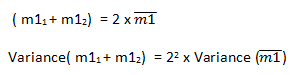
We know the variance on the left hand side is 50. The variance of our average value is therefore 50/4 = 12.5.
The standard deviation is the square root of the variance, therefore we have:
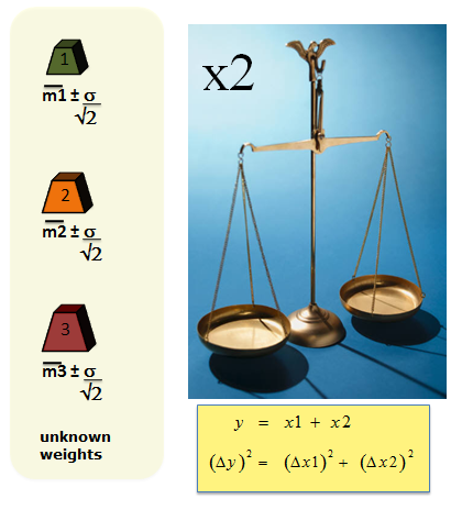
Returning to our estimation of 3 unknown weights, if we perform a total of 6 measurements then we can achieve results with a precision of σ/√2.
But by exploiting the above behaviour of how variances propagate through the measurements and the calculations we could devise a more efficient albeit less intuitive experiment. Instead of measuring the 3 weights individually, we weigh them in combinations:
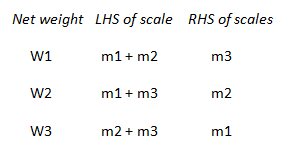
This results in 3 simultaneous equations that can be solved. The outcome is a precision of σ/√2 for each of the 3 weights.
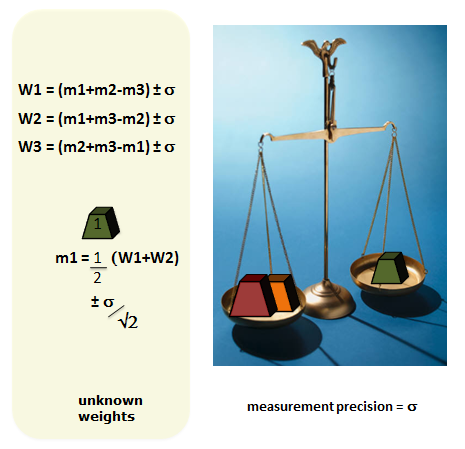
Note that we achieve this precision by performing only 3 measurements – half the number required to achieve the same precision using a more intuitive one-at-a-time experimentation.
As an illustration of one of the calculations consider the weight m1. It is measured indirectly through the measurements W1, W2 and W3:
![]()
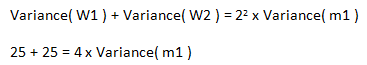
If we add W1 and W2 then:
![]()
hence![]() and
and
Consequently![]() and
and![]()
In these measurement examples I’ve considered discrete quantities. When we have variables that can measured on a continuous scale we have yet further decisions to make with regard to the experimental strategy. Again statistical thinking can guide us in a direction that is more efficient than perhaps more intuitive approaches.
Consider a simple situation where we expect a linear relationship between two variables, and the corresponding slope is the quantity that we wish to measure.
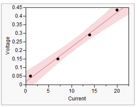
In this graph, the slope would represent the resistance of a resistor obeying Ohm’s Law.
The line can be estimated using the method of Least Squares.
This method also provides the calculations for determining the standard deviation of the slope (based on the same principles of propagation discussed earlier).
Yet whilst it is comforting to see a sequence of points falling along a line, if we know the relationship is linear, we can reverse-engineer the Least Squares method to determine the configuration of measurements that will yield the best precision.
Below we compare two experimental configurations:
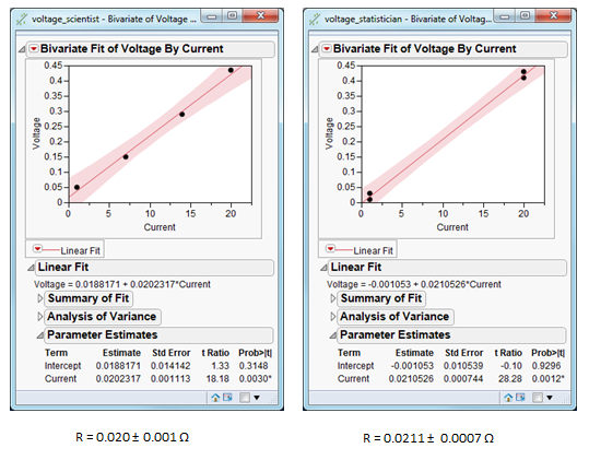
By understanding how our data is going to be analysed, the analysis can be reverse-engineered to maximise the information yield. This is the essence of statistically designed experiments.