In my last post I built a regression model with a single predictor variable. That variable represented the value of a single pixel from a 28×28 image of a hand written digit. In this post I will look at some model variations based on using a larger number of input variables.
Significant Pixels
One of the tasks I performed in my last post was to evaluate logistic models for each of the 784 pixels in the image. Here is a plot of the performance of all of those models:
![]()
There are 3 distinct groups of pixels. From each of these groups I have labelled the best performing pixels. They are: pixels 217, 515 and 657.
Using a utility script that I have written I can visualise the role of these pixels in differentiating between the digits 5 and 6:
![]()
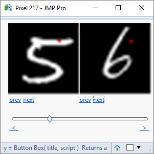
![]()
These pixels clearly identify different features associated with the pen strokes of the digits.
There were two other pixels that I identified (pixels 102 and 413). Their influence was not so strong but they seemed to represent further distinct groups:
![]()
![]()
If I construct a model that includes all these pixels as predictor variables I achieve a misclassification rate of less than 10% :
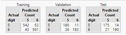

So now let me look at the problem from a different perspective. Instead of identifying the most influential pixels and creating a small model, I’m going to just use all of the pixel data:
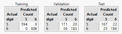
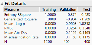
What I see is that the training misclassification rate improves but the test misclassification rate increases. This is a classic outcome that arises due to overfitting.
Overfitting
To illustrate the problem of overfitting I can run a script that incrementally add terms to the model to evaluate the effect of model complexity on the model performance:
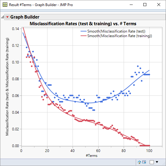
Adding complexity to a model allows it to increasingly describe nuances of the data – even if those nuances are just noise. So this means that the training performance continues to improve as the model size increases. For the test dataset however, there are 3 distinct phases.
First, model performance improves as additional terms are added to the model. Then there is a period where performance has levelled-out (between 30 and 60 terms) – the model has reached the point where additional terms deliver no improvement. This region of the graph also indicates to me the best level of performance that I can expect to achieve: a misclassification rate close to 0.05. In the final phase test performance decreases; the model is now describing features of the noise that are present in the training dataset but not the test dataset resulting in degraded predictive performance.
In doing this investigation I learn 3 things:
- It is naive to look for the best model.
- I expect to be able to find a model with a misclassification rate close to 0.05.
- I probably need to find a model with about 30 terms to achieve the above classification rate.
How do I find that model? Easy right? I’ve already built it in creating the data for the graph. The problem is that I made a decision to add pixels in a particular order based on a reasonable heuristic but not one designed to try and optimise performance. If I want to add terms sequentially to a model in a way that is designed to improve performance at each step then I should look at using stepwise regression.
But there is also a nagging doubt: adding more terms to the model feels like it should improve it. Perhaps the overfitting is a feature not of the model but of my test environment; perhaps large models perform poorly not because of their inherent size but because they are large relative to the amount of data that I am using the build the model. Put another way: if I were to use more data, could I build more complex models with better predictive performance? To answer this question I can build a graph similar to above, but investigating quantity of data rather than the number of terms.
And finally, returning to the idea of selecting the terms for a model. If a term is not in the model it’s like scaling the parameter estimate by zero whereas if it is in the model it’s like scaling the parameter by one. But there is no reason why the scaling has to be binary – why I can’t I scale it by 0.5. Think of it as a “Schrodinger Cat” model: the term is half in and half out! And when we talk about models having too many terms, perhaps the solution is not to throw out individual terms out but rather, to shrink the size of all the parameters so that their sum is reduced. I can investigate this approach to model building using generalized regression.
So in my next post I will look at using stepwise regression and generalized regression. Below I will wrap up this post by looking at the impact of adjusting the amount of data available for training the model.
The Effect of Data Quantity on Model Training
I want to create a graph similar to the one above, but where the x-axis will represent to amount of data used in the training dataset. To do this I need use a model of fixed size: I’ll take 95 terms. In order to increase the amount of data I’ll refer back to my source data that contained in excess of 10,000 images. By the time I’ve partitioned the data into training, validation and test datasets I still have over 6,000 training images that I can use. Using the ‘exclude’ property of rows I can control how much of this image data will be used when training a model.
Here’s the script that will do the hard work for me:
|
1 2 3 4 5 6 7 8 9 10 11 12 13 14 15 16 17 18 19 20 21 22 23 24 25 26 27 28 29 30 31 32 33 34 35 36 37 38 39 40 41 42 43 44 45 46 47 |
// data sorted so that rows 4537 onwards are the training dataset dt = Current Data Table(); dt << Show Window(0); nr = NRows(dt); startRow = 4537; lstFactors = {"Pixel544", "Pixel516", "Pixel515", "Pixel656", "Pixel658", "Pixel657", "Pixel545","Pixel659", "Pixel488", "Pixel487", "Pixel517", "Pixel543", "Pixel655", "Pixel486","Pixel660", "Pixel217", "Pixel216", "Pixel573", "Pixel574", "Pixel218", "Pixel244","Pixel514", "Pixel219", "Pixel575", "Pixel654", "Pixel626", "Pixel215", "Pixel243","Pixel245", "Pixel246", "Pixel489", "Pixel546", "Pixel625", "Pixel458", "Pixel459","Pixel572", "Pixel101", "Pixel189", "Pixel627", "Pixel685", "Pixel102", "Pixel661","Pixel518", "Pixel686", "Pixel190", "Pixel247", "Pixel576", "Pixel242", "Pixel220","Pixel188", "Pixel413", "Pixel687", "Pixel628", "Pixel653", "Pixel129", "Pixel100","Pixel441", "Pixel460", "Pixel485", "Pixel597", "Pixel214", "Pixel457", "Pixel684","Pixel271", "Pixel490", "Pixel547", "Pixel130", "Pixel191", "Pixel270", "Pixel469","Pixel248", "Pixel662", "Pixel272", "Pixel414", "Pixel442", "Pixel633", "Pixel128","Pixel542", "Pixel624", "Pixel550", "Pixel577", "Pixel596", "Pixel632", "Pixel683","Pixel273", "Pixel385", "Pixel187", "Pixel192", "Pixel430", "Pixel549", "Pixel103","Pixel384", "Pixel412", "Pixel431", "Pixel513"}; lstNumData = {}; lstTrnRates = {}; lstValRates = {}; lstTstRates = {}; For (i=1400,i<=6000,i=i+200, dt << Clear Row States; startExcluded = startRow + i; excludedRows = startExcluded::nr; dt << Select Rows(excludedRows); dt << Exclude; fm = dt << Fit Model( Y( :digit ), Effects( Eval(lstFactors) ), Validation( :Validation ), Personality( "Nominal Logistic" ), Run( Likelihood Ratio Tests( 0 ), Wald Tests( 0 ), Logistic Plot( 0 ) ), SendToReport( Dispatch( {}, "Fit Details", OutlineBox, {Close( 0 )} ) ) ); model = fm << Get Scriptable Object(); rep = model << Report; mat = rep[NumberColBox(15)] << Get As Matrix; trainingRate = mat[6]; mat = rep[NumberColBox(17)] << Get As Matrix; valRate = mat[6]; mat = rep[NumberColBox(19)] << Get As Matrix; testRate = mat[6]; InsertInto(lstNames,cName); InsertInto(lstTrnRates,trainingRate); InsertInto(lstValRates,valRate); InsertInto(lstTstRates,testRate); InsertInto(lstNumData,i); rep << Close Window; ); dt << Clear Row States; dt << Show Window(1); New Table("Result #Data", New Column("# Training Data Rows", numeric, Set Values(lstNumData)), New Column("Misclassification Rate (training)", numeric, Set Values(lstTrnRates)), New Column("Misclassification Rate (validation)", numeric, Set Values(lstValRates)), New Column("Misclassification Rate (test)", numeric, Set Values(lstTstRates)) ) |
And this is the output:
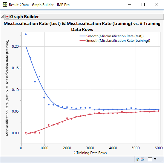
There are a number of interesting features about this graph:
- Too few data points degrades the predictive performance (as indicated by the curve for the test data)
- There comes a time where additional data fails to improve predictive performance (~3000 data points)
- A perfect training model results from too few data points
- There is a clear consensus that that good model performance asymptotes to a misclassifcation rate of 0.05
If you recall, I was wondering whether the poor performance of my larger models was really down to overfitting or due to lack of training data, and whether larger models would be more useful. My earlier graph was based on 2000 data points (of which only 1200 were training data) . The conclusion I arrive at is that the poor performance was due to lack of data, but that with more data and larger models I’m unlikely to see a significant improvement on performance (I had a model with 30 terms with a misclassification rate close to 0.05).
I would like to see less divergence between the performance of the test and training datasets – to achieve that I would like 3000 training images – if only 60% of my data is used for training then I should increase the amount of data I am using to 5000 data points. I’m able to do that – I have almost 12000 data points. Why not just use all the data? When I investigated the effect of the number of terms I built a model with 1 term, then 2 terms, … up to 100 terms; that’s over 5,000 models – so keeping the data size down is one way to shorten the required computation time.
One thought on “Logistic Regression pt. 2”