There are two main classes of model for time series data – autoregressive (AR) and moving average (MA). The generalisation of the two is referred to as ARIMA – autoregressive integrated moving average. These models are sometimes referred to as Box-Jenkins models, but more accurately the term “Box-Jenkins” refers to a methodology for model selection.
The Nature of Time Series
A time series is a one-dimensional set of data sequenced by time. Based on this sequence time series analysis seeks to make inferences about future values. To do this a model must be constructed, and that model needs to exploit the serial dependencies within the data. This is very different to ordinary least squares where observations are assumed to be independent of each other.
If it is a hot day today then you’ll probably have a reasonable expectation that it will be hot tomorrow
There are two mechanisms (or processes) through which dependencies can arise. I’ll try and illustrate the first with respect to the weather. If it’s a hot day today then you’ll probably have a reasonable expectation that it will hot tomorrow (this probably works if you live in California, if you live in the UK replace ‘today’ and ‘tomorrow’ with ‘now’ and ‘in one hours time’!).
If this expectation is correct then today’s weather will also be related to yesterdays weather; logically therefore tomorrow’s weather is dependent on the weather of both today and yesterday. This leads to an autoregressive model where there is correlation with the prior data points. The parameters of an autoregressive model quantify these levels of correlation. We might expect the correlation to weaken as we look further back in time. Later we’ll see that this manifests itself as a decaying envelop containing correlation values.
That paragraph can be summarised much more effectively with mathematical notation:

This is an autoregressive model of order p.
As with any statistical model it contains signal (y) components and noise (ε) components. With the autoregressive model the value of one data point is dependent on the prior values of the signal whereas with the a moving average model the value is dependent on the prior values of the noise:

Model Identification
This can be performed by looking at an autocorrelation function and a partial correlation function.
One, if not the, key step in the creation of a time series model is to determine whether an autoregressive (AR) or moving average (MA) model should be used to explain the serial correlation within the data. This can be performed by looking at an autocorrelation function (ACF) and a partial correlation function (PACF).
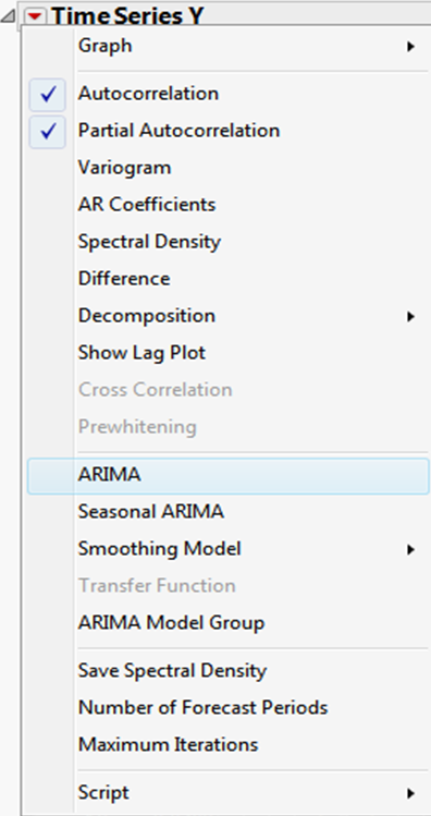
Fortunately I can explain the utility of these functions using the graphical output of the JMP Time Series platform without any further reference to the underlying mathematics!
Let’s take some data that I know to be a second-order autoregressive average model (I know because I have a script to generate the data). Here is the body of the output from the JMP Time Series platform:
On the left there is an autocorrelation function (ACF) and on the right there is the partial autocorrelation function (PACF). It’s not my intention to go into the mathematics. The way we use these graphs is similar to residual analysis on ordinary regression.
If I have an autoregressive model then I expect the magnitude of the ACF correlations to decay smoothly as the lag increases. At the same time I expect the PACF correlations to abruptly reduce at the point where there is no further significant correlation. For this data there are three large correlation bars on the PACF. But note the third bar corresponds to a lag of 2 not 3. The first bar represents a lag of zero – the correlation of a data point with itself (do I really want to see this?).
Now let’s look how the output differs for a second order-moving average model.
The exponential decay of the ACF function, indicative of a moving average process, is not present. For an autoregressive model, it is is ACF rather than the PACF that indicates the order of the model.
Building the Model
I will build a model based on the last set of data, where the inspection of the correlations leads me to postulate a second order moving average model.
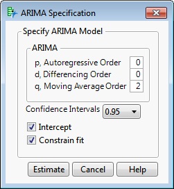
Once the order of the model is specified JMP will estimate the model terms.
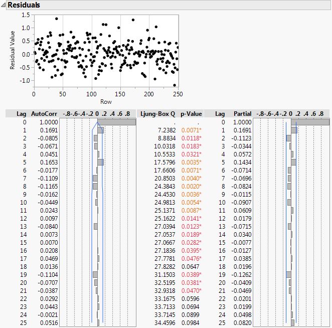
Now I have a model I want to look at correlation plots again, but this time with respect to the residuals. My goal is to generate a set of residuals that exhibit no correlation. In this example it looks like I have achieved my goal:
Whether we want to assess model improvements as we iteratively refine the model, or whether there are competing models with different structure, JMP provides a table of model performance metrics to aid model comparison:
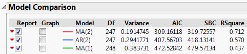
The above table shows that I was correct to select an MA(2) model as opposed to an AR(2) model, and that the second order model is significantly better than a first order model.
In general a time series model may contain both AR and MA components. But both of these model types are based on a time series with constant mean. This requirement is violated if there is either a trend or seasonal variation.
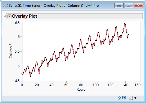
Time series model are typically built up iteratively to take account of the diffferent components. Trends and seasonality are taken into a account by a process known as differencing.
new to version 12 of JMP
Version 12 of JMP introduces new decomposition methods to remove trend and seasonal effects including the X-11 method developed by the US Bueau of the Census.
If you have opened the Time Series platform in the past and been intimidated by the output then I hope that this has served as a useful introduction to the graphical output that is produced by JMP in support of Box-Jenkins methodology. Why not take some time to take another look, and check out the features new to version 12 of JMP, found under the decomposition menu.
klass webbplatsen . Tack .